 Englisch Englisch |
U-tube oscillator |
|
1.0 Introduction 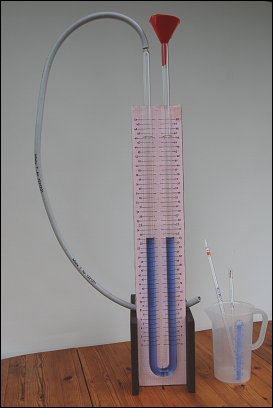
A slender, tall tree, blown by the storm, does not break off because it retreats elastically and, when the wind subsides a little, causes vibrations. Is this a whim of nature or is there a principle behind it that is not recognizable at first glance? We encounter vibrations at many places in daily life.
Everyone knows the children's swing. But also the string of a guitar, a tuning fork or the membrane of a drum produce hardly visible vibrations, which stimulate the air to sound waves and create the auditory impression via our eardrum in the ear.
The technology uses the pendulum or balance wheel to produce accurate timers, or the swinging suspension to increase driving comfort in a motor vehicle. Even molecules, the atoms in a crystal lattice and even the atomic nuclei perform vibrations and thus store energy.
The principle of vibration is always the same:
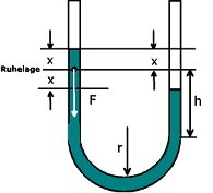
Elastic objects, which are brought out of equilibrium by an external force, vibrate when they respond to the external excitation with a backward, location-dependent force. Backward means that the force exerted by the object acts opposite to the direction of the stimulating force. Location-dependent here means that as further the object is deflected from its equilibrium position, as greater is the response force.
With the U-tube oscillator you should experimentally measure different physical quantities that determine a vibration. In this experimental setup you can learn a lot about the concept of vibration. And once you understand the general principle, you can apply it to many different areas of physics.
While experimenting, you will also learn a lot about measurement technology. First of all, a meaningful execution of the experiments is a prerequisite for good results. With every measurement, measurement inaccuracies occur that you cannot avoid. For example, if you let several people measure the seat height of a chair, you get different results (46.3 cm, 46.2 cm, 46.7 cm, 46.55 cm, 45.9 cm...). The measured values scatter around a certain value, the mean value, which here is 46.33 cm. The range in which the measurement results lie, here ± 0.4 cm, is called measurement uncertainty. If you can specify the range of measurement uncertainty, you are able to make a statement about the accuracy of your measurement. Certainly, one goal is to make this area as small as possible.
2.0 Experimental setup The experimental setup consists of a U-tube made of glass with a leg length of 70 cm. The U-tube is filled with water or another suitable liquid. Furthermore, the following parts are available:
Please check that all items are present before starting your experiments.
3.0 Definitions and terms A vibration is a periodic movement. In this example, a column of liquid vibrates in a U-tube. There is a fixed physical quantity for this movement: the oscillation duration, which describes the movement and depends on the structure of the U-tube and the properties of all materials used.
The duration of oscillation is the time it takes for the deflected liquid column to return to the same state. These can be any heights, but also the maximum hight positions in the U-tube. The number of oscillations that the liquid column performs in one second is called frequency and is measured in units [1/s] or Hertz [Hz]. If the system is left to itself, it usually oscillates at a very characteristic frequency, such as a pendulum clock. This frequency is called natural frequency.
The largest deflection of an oscillation is called amplitude.
The flow velocity is not constant during oscillation and is influenced by friction, e.g. on the pipe wall. This friction causes the amplitude to decrease over time. After some time, the state of equilibrium, namely the resting position, is restored.
4.0 First observations It is best to do a trial phase first. First, fill the U-tube about halfway with water. Deflect the liquid column out of its equilibrium position by blowing in or by suction and let it vibrate.
You now have an idea of what happens to the liquid. But your experiment should be more precise. Good scientists first describe your experimental setup and then what and how you measured. An important scientific tenet is the verifiability of your results by others. So you should now be able to generate real measured values and also say how good they are.
5.0 General information Quantitative measurements make experiments comparable. This makes it possible to check predictions from theory. With every measurement, however, measurement inaccuracies arise, which of course have nothing to do with incorrect work. Only by specifying the size of these inaccuracies can the quality of the measured values be assessed.
The following measurement inaccuracies may occur:
6.0 Information on vibration duration It has already been mentioned in the introduction: The duration of oscillation is the time it takes for the deflected liquid column to return to the same state. These can be any heights in the U-tube.
6.1 Tasks for vibration duration 6.2 Tasks for the variation of liquid components It seems obvious that the type of liquid has an influence on the duration of the oscillation. To check this, you have to carry out measurements on liquids with different properties.
As you have already stated above, density and toughness determine the property of the liquid. If the selection criteria are also the ease of manufacturability, the health risk and the cleaning of the U-tube, then sugar solutions in different concentrations are suitable for experimentation.
7.0 Information on vibration amplitude 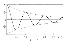
During the first measurements on the U-tube you noticed that the amplitude of the oscillation decreases over time. This oscillation is also called damped oscillation. In the adjacent figure (from literature) you can see an example of how the amplitude of a liquid oscillation decreases with time, which was deflected by the value x at the beginning. The reason for the amplitude decrease of the oscillation is the friction of the liquid on the pipe wall and in itself. Due to friction, vibrational energy is lost, the amplitude of the oscillation is dampened. Depending on the degree of attenuation, three cases can be distinguished:
8.0 Energy considerations at the U-tube oscillation A harmonic oscillation occurs when - as already explained in the introduction - location-dependent, driving forces are present in a system. In the U-tube oscillator, gravity is involved as a driving force. After excitation of the oscillation, potential energy of the liquid column is converted several times into kinetic energy and vice versa. With each oscillation, some of this energy is lost due to friction.
8.1 Tasks on the different forms of energy of U-tube vibration 9.0 Information on the form of flow For a flowing medium in the pipe, there is basically the "laminar", the "turbulent" and "periodic" flow form. The characteristic of a laminar flow is a uniform velocity profile over the entire length of the pipe. Perpendicular to it, i.e. on the circular cross-section of the tube, the velocity of the liquid particles at the edge of the pipe is almost zero and maximum at its center. The cause of this profile is the toughness or viscosity of the liquid. Viscosity describes how much a flowing medium deforms under the action of a force. Tar or honey have high viscosity values, while water or gases such as air have low viscosity values. In the particle model, the viscosity can be attributed to attractive forces or generally interactions between the molecules.
Characteristics of a turbulent flow are uneven vortex formations in the liquid, which are caused by small disturbances at the edge of the pipe or in the flow cross-section. In nature, every torrent forms a turbulent current. Turbulence only starts at a certain limit velocity, whereby flow energy is stored in the vortices. This "vortex energy" is no longer available to the oscillation, the turbulent oscillating system is therefore more damped than the laminar system. Through rocking processes, a turbulent flow can become chaotic; their behaviour is then difficult to predict.
The English physicist Osborne Reynolds made important discoveries about currents at the end of the 19th century. He found that the behavior of all currents can be described using a single dimensionless number, the Reynolds number Re. It is a measure of whether random small disturbances grow into vortices and turbulence or subside again. For the flow of liquids in pipes with circular cross-section: Re = ρ di v / η. It can be seen that at a given density ρ of the fluid and given diameter di of the tube, the Reynolds number increases with increasing velocity v and decreasing viscosity η. As soon as the Reynolds number exceeds a critical value Rec, a previously laminar flow can become turbulent. The critical Reynolds number for a flow in the pipe is Rec = 2320. By changing the formula, the critical velocity vc can be determined from which turbulence is to be expected.
In the case of periodic flow, in addition to the local velocity profile, there is also a temporal change: the amount of velocity at any point in the liquid increases and decreases within fixed time intervals. In the case of liquid column oscillation in the U-tube, the velocity of the fluid changes from zero in the reversal points (bottom, top) to a maximum value in the middle of the oscillation path (zero crossing).
9.1 Tasks for the flow form of vibration 10.0 Information on excited vibration With the motor, the connecting rod gearbox (it converts a rotary movement into a linear movement) and the air pump, the liquid column can be deflected not only once, but periodically. The air volume in the coupled U-tube is compressed and exerts pressure on the liquid column. The number of revolutions of the motor can be varied by changing the motor voltage within a sufficient range. The liquid column can be excited with adjustable oscillation duration or frequency.
If the frequency of the excitation is varied, the oscillating system responds with different amplitudes. This has a maximum at the natural frequency of the system. This is referred to as resonance. The energy stored in the system is greatest in the case of resonance. The ratio of stored energy to loss energy is called quality Q of the vibrating system.
10.1 Tasks for excited vibration 11.0 References |
|
| Copyright by Hans Joachim Ilgen seit 1950 | |